
The One More Paradox
Ever felt the odds seem so favourable in a bet or at a casino or while trading forex ? But then why do people prefer to stay out of such situations. Are they wise ? Let's find out.

Imagine starting with $100 and engaging in a game where each coin flip determines the fate of your wealth. If the coin lands on heads, your current wealth increases by 80%; if it lands on tails, it decreases by 50%. For example, you flip heads, so your $100 is multiplied by 1.8. Heads again, so your $180 is multiplied by 1.8. Then tails, so your $324 is multiplied by 0.5 And so on…
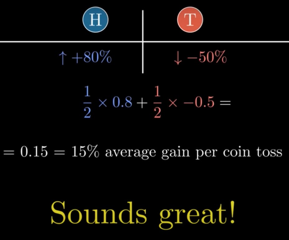
You have a ½ chance of 0.8 gain + a ½ chance of -0.5 loss. That’s an arithmetic mean of 0.15; a 15% average gain per coin toss.
Would you play this game? If yes then let’s simulate a million people, each starting with $100 and playing 50 rounds. A graph of their average wealth. As expected, their average grows exponentially. However, their median and mode plummet to a measly $7.2.
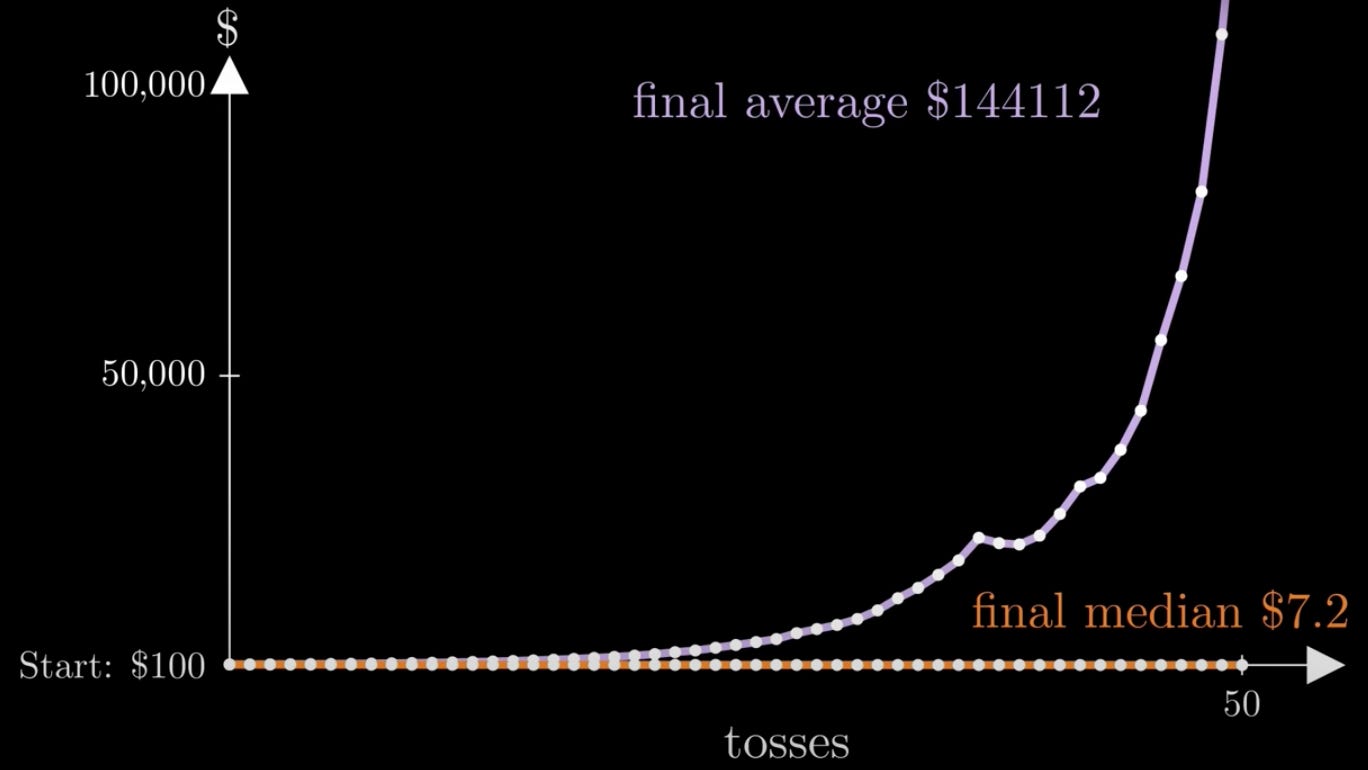
This is called a non-ergodic system because the population average is different from the median outcome of individuals. But how is the median this low?
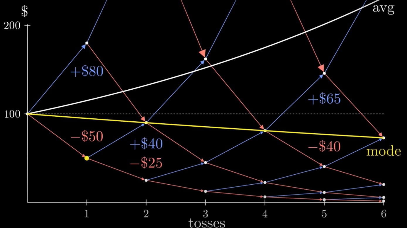
Let’s visualize the problem. So, we start here, with $100. We flip heads and multiply by 1.8, or tails and multiply by 0.5. From each of these two points, we can flip heads or tails. Note that flipping 1 head and 1 tail already drops us down to $90. … The average increases, pulled up by the luckiest outliers.
The mode slopes downward. This is shocking since every coin flip seems favourable. Starting out, we can gain 80 or lose only 50. Here we can gain 65 or lose only 40. Here we can gain 40 or lose only 25. This is called the “ Just One More Paradox ''. Each individual flip seems good, but the outcome is bad. This paradox applies to everything from gambling to social relationships to life decisions. That’s the beauty of math. The paradox arises due to the Multiplicative nature of the game. Each flip Multiplies our entire wealth by some factor. The lower we go, the less we can gain.
What if we didn’t bet our entire wealth on each coin flip?
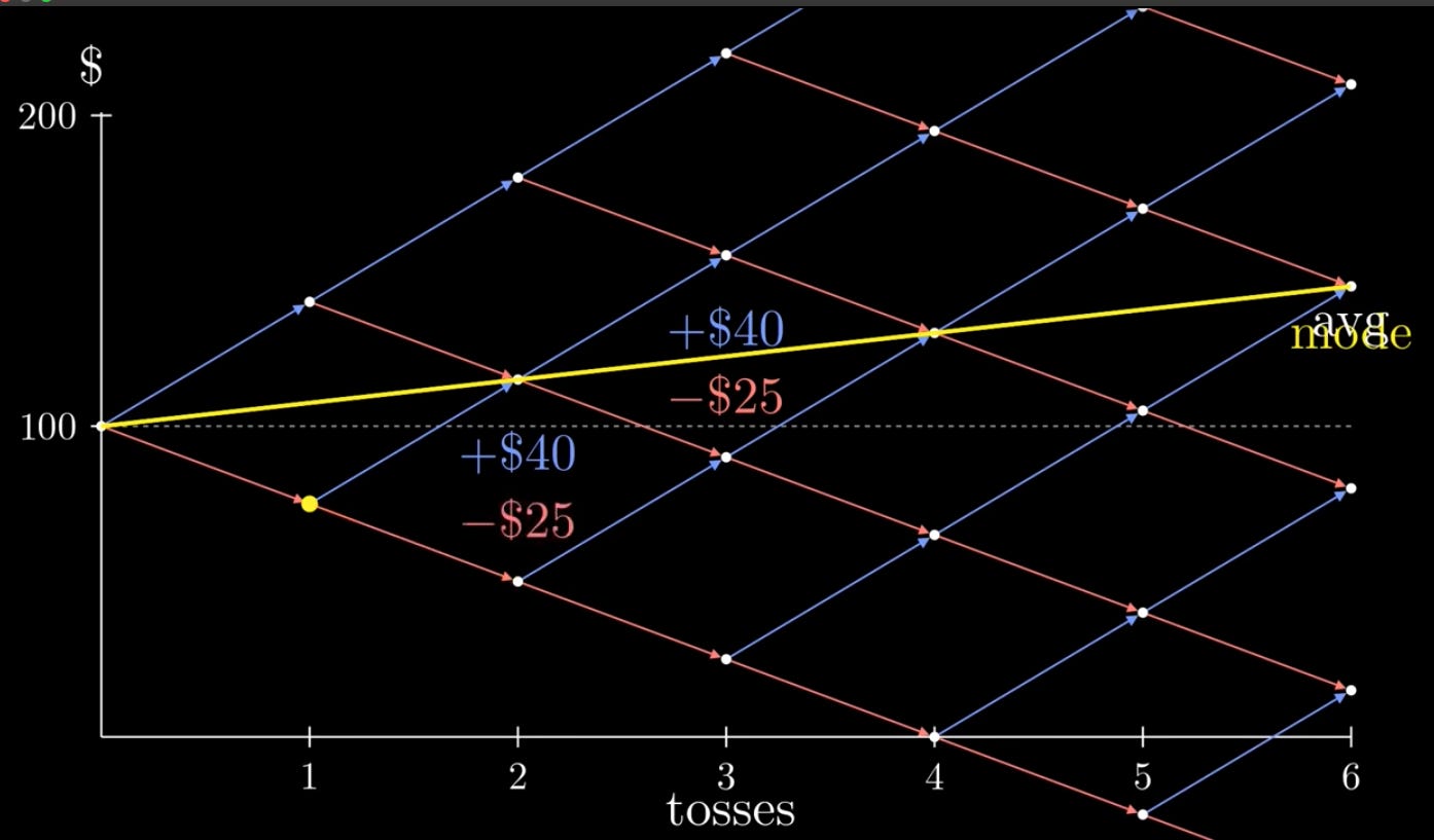
Let’s try betting only a fixed amount of 50 dollars on each coin flip. This is an Additive way to play the game. We simply changed our strategy. Now heads always give 40 dollars, and tails always subtract 25 dollars, no matter where we are. Our mode now slopes upwards and equals the average. That’s great! But this strategy isn’t perfect. How much should you bet if you have less than 50 dollars? What if you reach 1000 dollars? Should you raise your bet size?
You might be wondering: what if we always only bet a fraction of our wealth - say ⅕, or maybe 1/10.
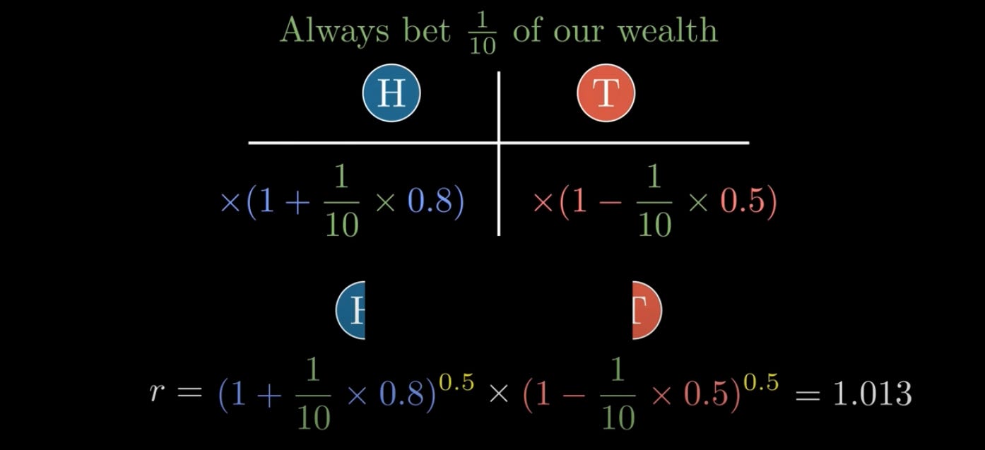
On heads, our wealth will be multiplied by 1 plus .8, times 1/10. On tails, our wealth is multiplied by 1 minus .5 times 1/10. Or simply… If we flip 1 head, and 1 tail, it would look like below. Remember, our mode and median is flipping half heads and half tails. This expression gives us the expected mode growth rate per coin flip! The mode will be multiplied by 1.013 per coin flip, which is a net gain. By the way, this is called a geometric mean. But is betting 1/10 of our wealth optimal? Why not 1/15 or ⅕?
To answer this question, we can start by generalizing our equation. Let’s say F is the fraction of wealth we’re betting, B is the gain, A is the loss, and P & Q are the probabilities of heads and tails. Now let's substitute those variables in. The x-axis represents the fraction of wealth bet. The y-axis represents the mode growth rate.
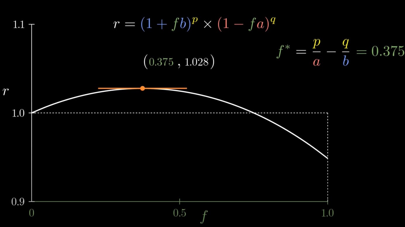
When f=0, we’re not betting anything,so there’s no change in wealth, and our growth rate is 1. When f=1, we’re betting our entire wealth.
Highest growth rate occurs where this curve’s slope is flat. We can use calculus to find where this is. If you don’t yet know calculus, it’s fine if you zone out for the next few seconds. We logarithmically differentiate with respect to r and set dr/df to zero, then solve for f. Ok, zone back in.
This equation tells us at what value of F the curve’s peak occurs. Plugging in our values gives 0.375. That’s the fraction of our wealth we should bet to maximize growth rate for these set of values. At this fraction, the mode growth rate is 1.028 per coin flip.
Let’s run our simulation again, having a million people each bet only .375 of their wealth. Here’s the average…
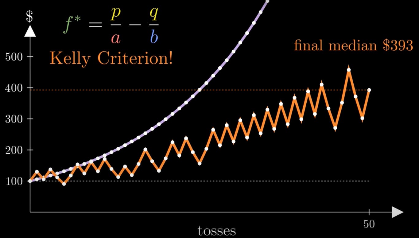
And yay! This time the median increases steadily! All thanks to this equation, called the Kelly Criterion. Described in 1956 by John Larry Kelly Jr. It is widely used by investors, specifying what fraction of wealth to bet to maximize growth rate.
At the end coming back to the question at the start honestly, there is no right or wrong, personally knowing this makes me comfortable in risking capital with correct returns. By acknowledging the disconnect between individual perceptions and aggregate realities we can make better decisions.
If you liked reading this hit the button below for more such interesting articles & feel free to share this.
Sources & References
Great ergodicity economics blog post by Jason Collins: https://www.jasoncollins.blog/posts/e...
A great video on youtube by Marcin Anforowics helped with visualisation.
Related article: Myers, J. K. (2021). Multiplicative Gains, Non-ergodic Utility, and the Just One More Paradox (with Supplemental Information). https://www.researchsquare.com/articl...
Interesting article 👍